Example Interrupted Time Series (ITS) with pymc models#
This notebook shows an example of using interrupted time series, where we do not have untreated control units of a similar nature to the treated unit and we just have a single time series of observations and the predictor variables are simply time and month.
import arviz as az
import pandas as pd

import causalpy as cp
%load_ext autoreload
%autoreload 2
%config InlineBackend.figure_format = 'retina'
seed = 42
Interrupted Time Series (ITS) Example#
Load data
df = (
    cp.load_data("its")
    .assign(date=lambda x: pd.to_datetime(x["date"]))
    .set_index("date")
)

treatment_time = pd.to_datetime("2017-01-01")
df.head()
| month | year | t | y | |
|---|---|---|---|---|
| date | ||||
| 2010-01-31 | 1 | 2010 | 0 | 25.058186 |
| 2010-02-28 | 2 | 2010 | 1 | 27.189812 |
| 2010-03-31 | 3 | 2010 | 2 | 26.487551 |
| 2010-04-30 | 4 | 2010 | 3 | 31.241716 |
| 2010-05-31 | 5 | 2010 | 4 | 40.753973 |
Run the analysis
Note
The random_seed keyword argument for the PyMC sampler is not neccessary. We use it here so that the results are reproducible.
result = cp.pymc_experiments.InterruptedTimeSeries(
    df,
    treatment_time,
    formula="y ~ 1 + t + C(month)",
    model=cp.pymc_models.LinearRegression(sample_kwargs={"random_seed": seed}),
)
Auto-assigning NUTS sampler...
Initializing NUTS using jitter+adapt_diag...
Multiprocess sampling (4 chains in 4 jobs)
NUTS: [beta, sigma]
Sampling 4 chains for 1_000 tune and 1_000 draw iterations (4_000 + 4_000 draws total) took 2 seconds.
Sampling: [beta, sigma, y_hat]
Sampling: [y_hat]
Sampling: [y_hat]
Sampling: [y_hat]
Sampling: [y_hat]
fig, ax = result.plot()
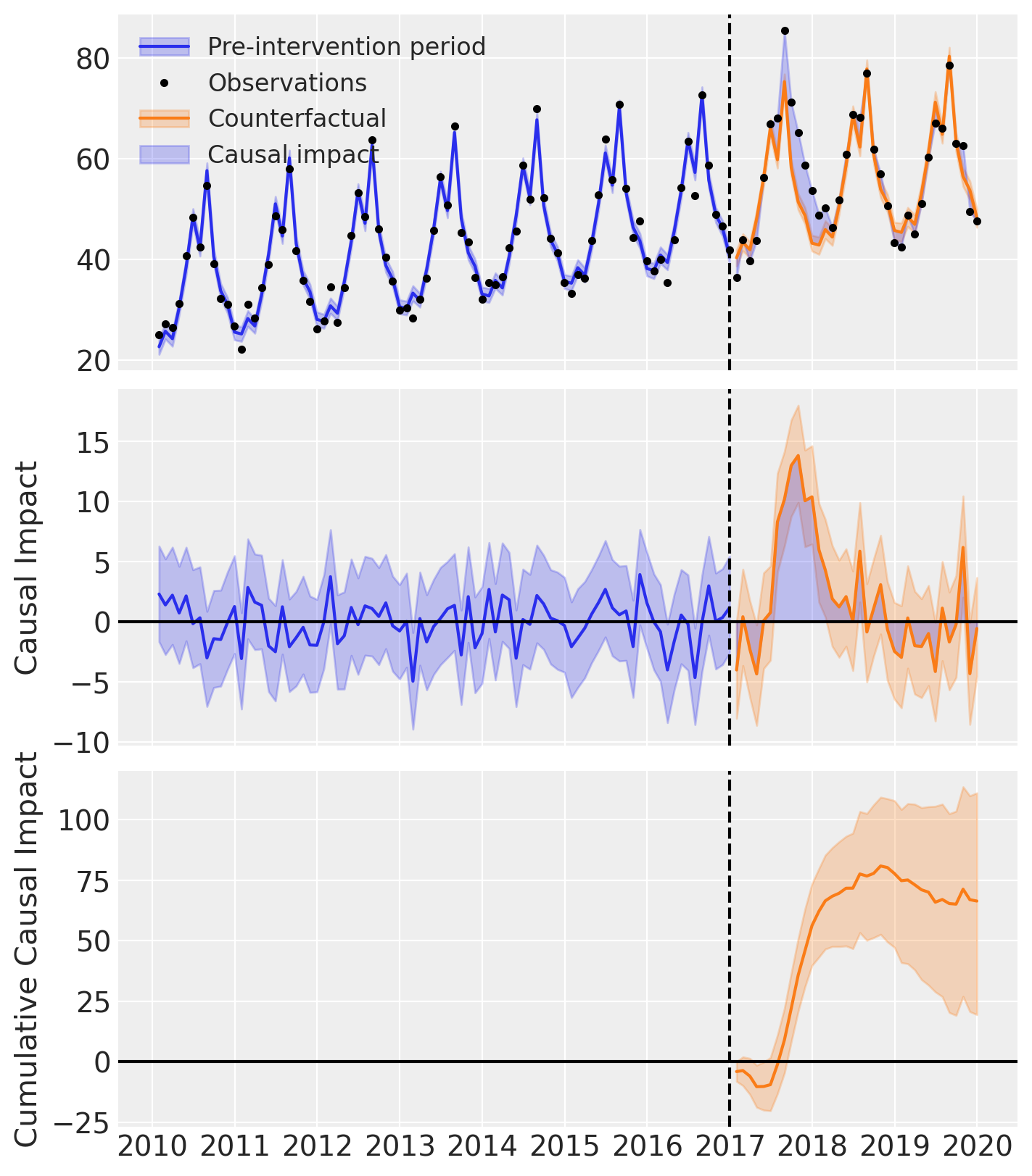
result.summary()
==================================Pre-Post Fit==================================
Formula: y ~ 1 + t + C(month)
Pre-intervention Bayesian $R^2$: 0.95 (std = 0.0086)
Model coefficients:
    Intercept       23, 94% HDI [21, 24]
    C(month)[T.2]   2.9, 94% HDI [0.88, 4.8]
    C(month)[T.3]   1.2, 94% HDI [-0.81, 3.1]
    C(month)[T.4]   7.1, 94% HDI [5.2, 9.1]
    C(month)[T.5]   15, 94% HDI [13, 17]
    C(month)[T.6]   25, 94% HDI [23, 27]
    C(month)[T.7]   18, 94% HDI [16, 20]
    C(month)[T.8]   33, 94% HDI [32, 35]
    C(month)[T.9]   16, 94% HDI [14, 18]
    C(month)[T.10]  9.2, 94% HDI [7.2, 11]
    C(month)[T.11]  6.3, 94% HDI [4.2, 8.2]
    C(month)[T.12]  0.59, 94% HDI [-1.4, 2.5]
    t               0.21, 94% HDI [0.19, 0.23]
    sigma           2, 94% HDI [1.7, 2.3]
As well as the model coefficients, we might be interested in the avarage causal impact and average cumulative causal impact.
Note
Better output for the summary statistics are in progress!
First we ask for summary statistics of the causal impact over the entire post-intervention period.
az.summary(result.post_impact.mean("obs_ind"))
| mean | sd | hdi_3% | hdi_97% | mcse_mean | mcse_sd | ess_bulk | ess_tail | r_hat | |
|---|---|---|---|---|---|---|---|---|---|
| x | 1.845 | 0.677 | 0.542 | 3.086 | 0.013 | 0.009 | 2631.0 | 3110.0 | 1.0 |
Warning
Care must be taken with the mean impact statistic. It only makes sense to use this statistic if it looks like the intervention had a lasting (and roughly constant) effect on the outcome variable. If the effect is transient, then clearly there will be a lot of post-intervention period where the impact of the intervention has ‘worn off’. If so, then it will be hard to interpret the mean impacts real meaning.
We can also ask for the summary statistics of the cumulative causal impact.
# get index of the final time point
index = result.post_impact_cumulative.obs_ind.max()
# grab the posterior distribution of the cumulative impact at this final time point
last_cumulative_estimate = result.post_impact_cumulative.sel({"obs_ind": index})
# get summary stats
az.summary(last_cumulative_estimate)
| mean | sd | hdi_3% | hdi_97% | mcse_mean | mcse_sd | ess_bulk | ess_tail | r_hat | |
|---|---|---|---|---|---|---|---|---|---|
| x | 66.436 | 24.359 | 19.508 | 111.108 | 0.476 | 0.337 | 2631.0 | 3110.0 | 1.0 |
Validating the model fit#
If we want, we can also conduct our parameter estimation on a portion of the pre-intervention period data, but leave a short validation period before the intervention. This allows us to see how well the model fits the data and could be a good idea if we have concerns about overfitting, or poor ability of the model to produce accurate forecasts thus a poor counterfactual prediction.
The intervention period was 2017-01-01, so we could choose whatever we think is appropriate as the validation time. Here we choose 2015-01-01, so that we have 2 years of observations which are not used in the parameter estimation that we can use to evaluate the ability of the model to forecast the outcome.
validation_time = pd.to_datetime("2015-01-01")
result2 = cp.pymc_experiments.InterruptedTimeSeries(
    df,
    treatment_time,
    validation_time=validation_time,
    formula="y ~ 1 + t + C(month)",
    model=cp.pymc_models.LinearRegression(sample_kwargs={"random_seed": seed}),
)
Auto-assigning NUTS sampler...
Initializing NUTS using jitter+adapt_diag...
Multiprocess sampling (4 chains in 4 jobs)
NUTS: [beta, sigma]
Sampling 4 chains for 1_000 tune and 1_000 draw iterations (4_000 + 4_000 draws total) took 2 seconds.
Sampling: [beta, sigma, y_hat]
Sampling: [y_hat]
Sampling: [y_hat]
Sampling: [y_hat]
Sampling: [y_hat]
Sampling: [y_hat]
result2.plot();
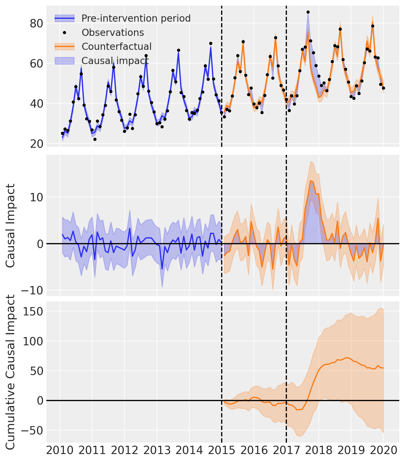
result2.summary()
==================================Pre-Post Fit==================================
Formula: y ~ 1 + t + C(month)
Pre-intervention Bayesian $R^2$: 0.94 (std = 0.011)
Validation Bayesian $R^2$: 0.92 (std = 0.022)
Model coefficients:
    Intercept       23, 94% HDI [21, 25]
    C(month)[T.2]   2.9, 94% HDI [0.65, 5.1]
    C(month)[T.3]   1.6, 94% HDI [-0.65, 3.9]
    C(month)[T.4]   6.9, 94% HDI [4.7, 9.1]
    C(month)[T.5]   14, 94% HDI [12, 16]
    C(month)[T.6]   24, 94% HDI [22, 26]
    C(month)[T.7]   18, 94% HDI [16, 21]
    C(month)[T.8]   33, 94% HDI [31, 35]
    C(month)[T.9]   15, 94% HDI [13, 17]
    C(month)[T.10]  9.1, 94% HDI [7, 11]
    C(month)[T.11]  4.9, 94% HDI [2.7, 7.1]
    C(month)[T.12]  -0.44, 94% HDI [-2.7, 1.8]
    t               0.21, 94% HDI [0.19, 0.24]
    sigma           1.9, 94% HDI [1.6, 2.3]